Extended figures with Codex links and additional visualizations for the publication Neuronal wiring diagram of an adult brain.
// video of all neurons coming on 10/2 at 11 am US ET (if you want a sneak peek try this link)
Figure 1
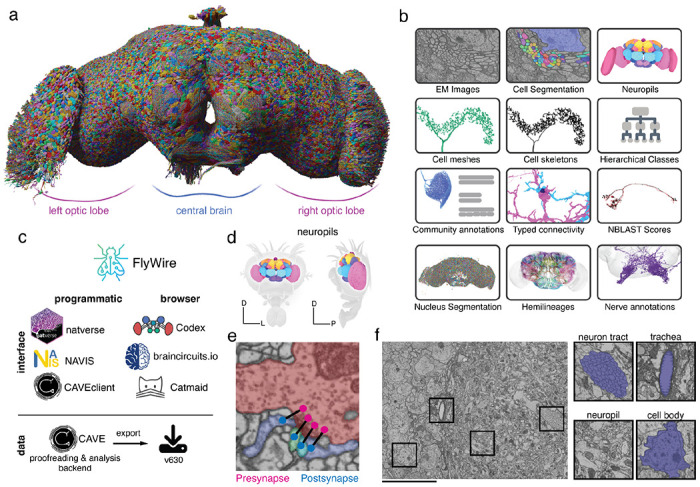
A connectomic reconstruction of a whole fly brain. figure
(a) All neuron morphologies reconstructed with FlyWire. All neurons in the central brain and both optic lobes were segmented and proofread. Note: image and dataset are mirror inverted relative to the native fly brain. (b) An overview of many of the FlyWire resources which are being made available. FlyWire leverages existing resources for EM imagery by Zheng et al.52, synapse predictions by Buhmann et al.45,46 and neurotransmitter predictions by Eckstein et al.47. Annotations of the FlyWire dataset such as hemilineages, nerves, and hierarchical classes are established in our companion paper by Schlegel et al. (c) FlyWire uses CAVE (in prep) for proofreading, data management, and analysis backend. The data can be accessed programmatically through the CAVEclient, navis and natverse168, and through the browser in Codex, Catmaid Spaces and braincircuits.io. Static exports of the data are also available. (d) The Drosophila brain can be divided into spatially defined regions based on neuropils110 (Ext. Data Fig. 1-1). Neuropils for the lamina are not shown. (e) Synaptic boutons in the fly brain are often polyadic such that there are multiple postsynaptic partners per presynaptic bouton. Each link between a pre- and a postsynaptic location is a synapse. (f) Neuron tracts, trachea, neuropil, cell bodies can be readily identified from the EM data which was acquired by Zheng et al.52. Scale bar: 10 μm
Explore all the connectome annotation types in Codex: https://codex.flywire.ai/app/annotations

Figure 2
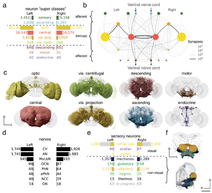
Neuron categories.
(a) We grouped neurons in the fly brain by “flow”: intrinsic, afferent, efferent. Each flow class is further divided into “super-classes” based on location and function. Neuron annotations are described in more detail in our companion paper by 44. The first public release is missing ~8,000 retinula cells in the compound eyes and four eyelets in one hemisphere which are indicated by hatched bars. (b) Using these neuron annotations, we created an aggregated synapse graph between the super-classes in the fly brain. (c) Renderings of all neurons in each super-class. (d) There are eight nerves into each hemisphere in addition to the ocellar nerve and the cervical connective (CV). All neurons traversing the nerves have been reconstructed and accounted for. (e) Sensory neurons can be subdivided by the sensory modality they respond to. In FlyWire, almost all sensory neurons have been typed by modality. The counts for the medial ocelli were omitted and are shown in Fig. 7b. (f) Renderings of all non-visual sensory neurons. Scale bar: 100 μm
Explore the Superclasses in Codex: https://codex.flywire.ai/app/annotations?for_attr_name=super_class&top_values=10000
Rendering of each of the 9 super classes. Images by Tyler Sloan and Amy Sterling.
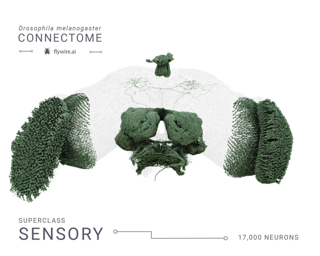
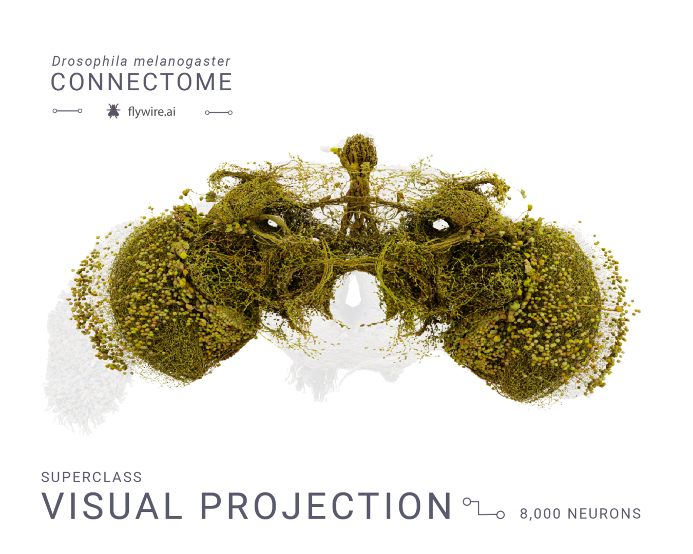
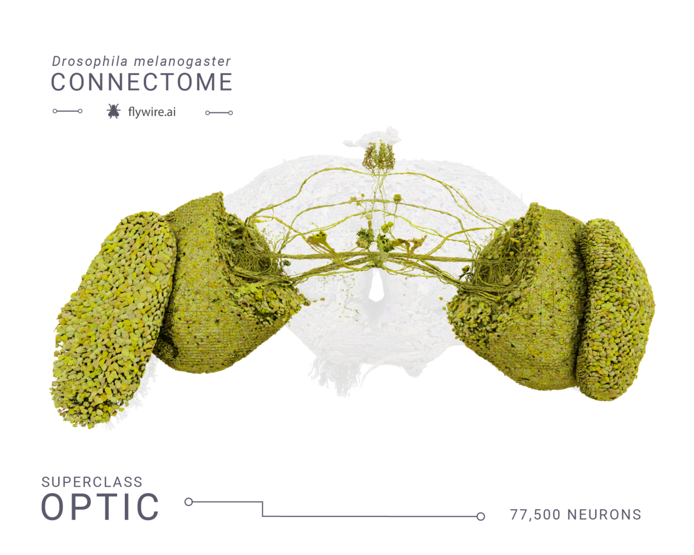
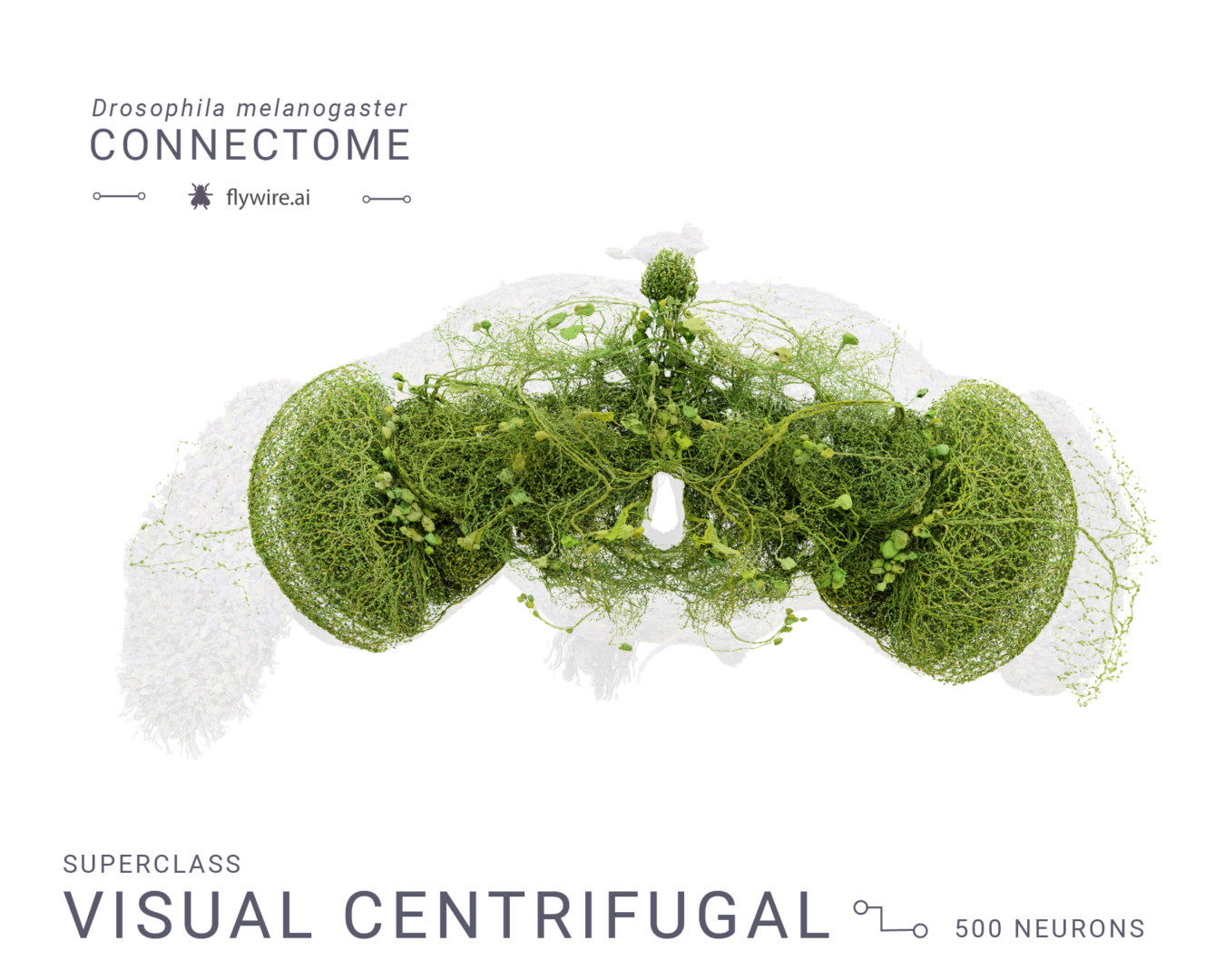
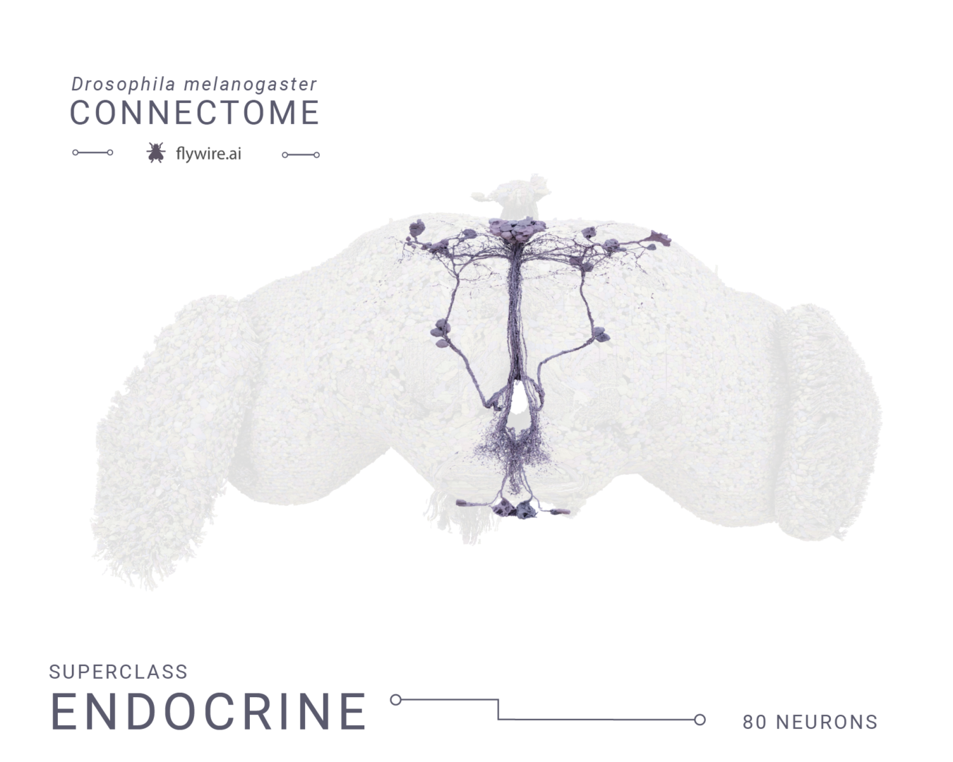
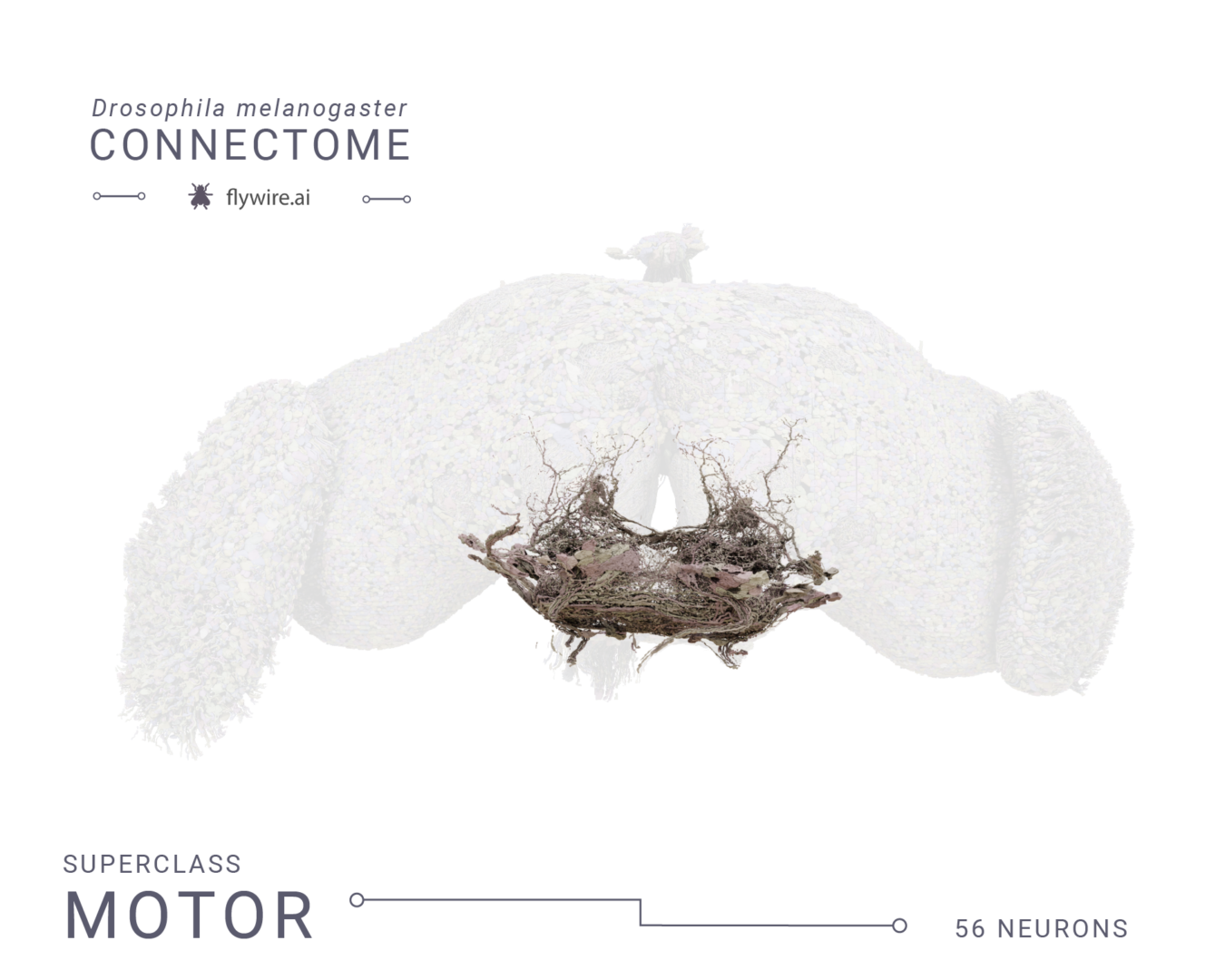
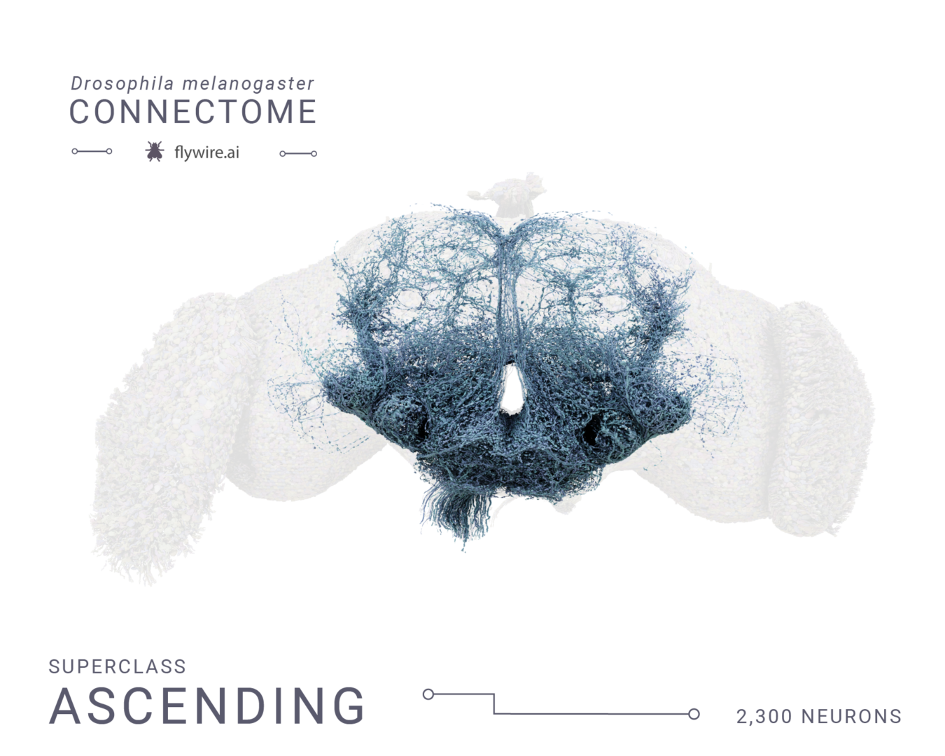
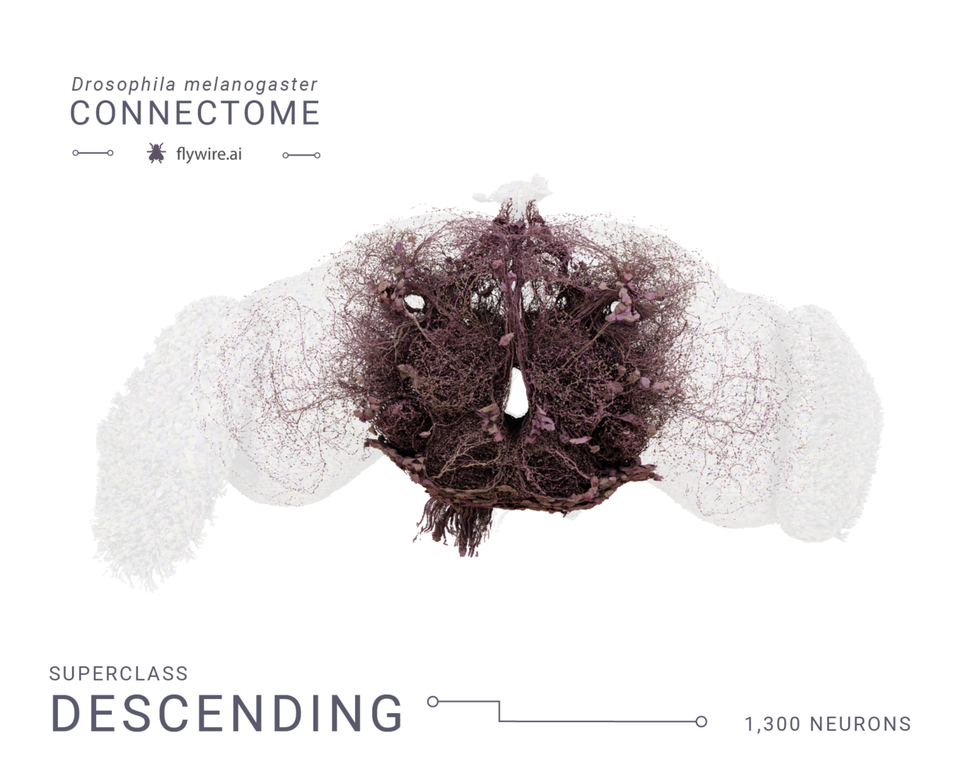
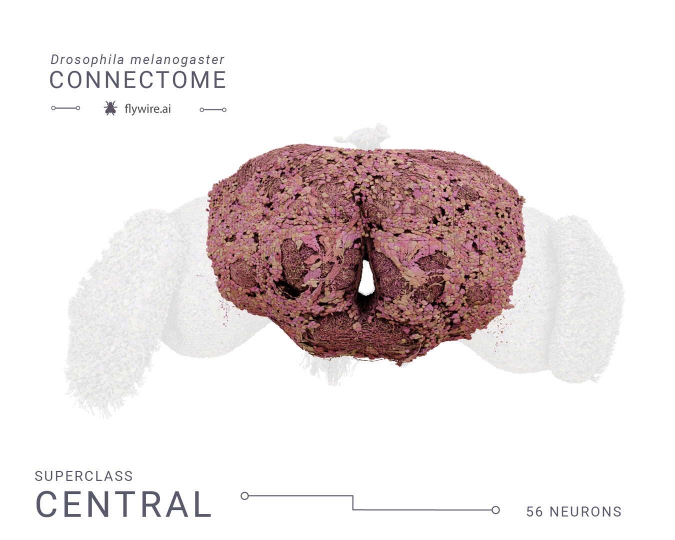
Figure 3
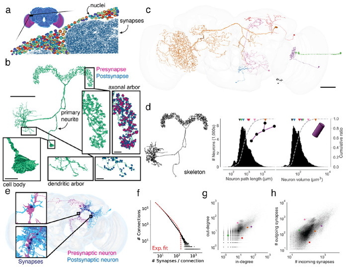
Figure 3: link
(a) The synapse-rich (synapses in blue) neuropil is surrounded by a layer of nuclei (random colors) located at the outside of the brain as well as between the optic lobes (purple) and the central brain (blue). (b) An LPsP neuron can be divided into morphologically distinct regions. Synapses (purple and blue) are found on the neuronal twigs and only rarely on the backbone. (c) We selected seven diverse neurons as a reference for the following panels. (d) The morphology of a neuron can be reduced to a skeleton from which the path length can be measured. The histograms show the distribution of path length and volume (the sum of all internal voxels) for all neurons. The triangles on top of the distributions indicate the measurements of the neurons in (b). (e) Connections in the fly brain are usually multisynaptic as in this example of neurons connecting with 71 synapses. (f) The number of connections with a given number of synapses and a fitted truncated power law distribution. (g) In degree and out degree of intrinsic neurons in the fly brain are linearly correlated (R=0.76). (h) The number of synapses per neuron varies between neurons by over a magnitude and the number of incoming and outgoing synapses is linearly correlated (R=0.80). Only intrinsic neurons were included in this plot. Scale bars: 50 μm (b, c), 10 μm (b-insets)
Take a tour of the neuron featured in 3b:
Explore the LPSP “Palm neuron” in Codex.
Animated version of figure 3e:
Explore all the synapses between these cells in Codex.
Figure 4
Neuropil projections and analysis of crossing neurons. link to figure
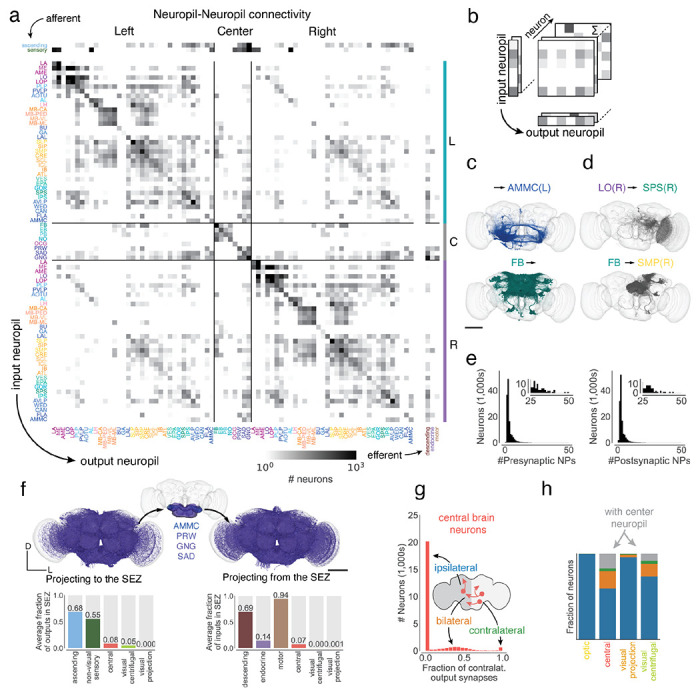
(a) Whole brain neuropil-neuropil connectivity matrix. The main matrix was generated from intrinsic neurons, and afferent and efferent neuron classes are shown on the side. Incoming synapses onto afferent neurons and outgoing synapses from efferent neurons were not considered for this matrix. See Ext. Data Fig. 4-1 for neurotransmitter specific matrices. (b) Cartoon describing the generation of the matrix in (a). Each neuron’s connectivity is mapped onto synaptic projections between different neuropils. (c) shows examples from the matrix with each render corresponding to one row or column in the matrix and (d) shows examples from the matrix with each render corresponding to one square in the matrix. (e) Most neurons have pre- and postsynaptic locations in less than four neuropils. (f) Renderings (subset of 3,000 each) and input and output fractions of neurons projecting to (N=11916) and from (N=7528) the SEZ. The SEZ is roughly composed of five neuropils (the AMMC has a left and right homologue). Average input and output fractions were computed by summing the row and column values of the SEZ neuropils in the super-class specific projection matrices. (g) Fraction of contralateral synapses for each central brain neuron. (h) Fraction of ipsilateral, bilateral, contralateral, neurons projecting to and from the center neuropils per super-class. Scale bars: 100 μm.
Explore the companion paper Network Statistics of the Whole-Brain Connectome of Drosophila
Figure 5
Optic lobes. Link to fig 5
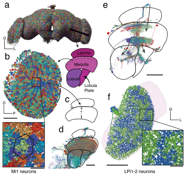
(a) Rendering of a subset of the neurons in the fly brain. A cut through the optic lobe is highlighted. (b) All 779 Mi1 neurons in the right optic lobe. (c) A single Mi1 neuron, (d) all neurons crossing through the column in c as defined by a cylinder in the medulla with 1 μm radius through it, and (e) all neurons sharing a connection with the single Mi1 neuron shown in (c) (≥ 5 synapses) – 3 large neurons (CT1, OA-AL2b2, Dm17) were excluded for the visualization. (f) The two LPi1-2 neurons in the right lobula plate (neuropil shown in background). Scale bars: 50 μm (b,c,d,e,f), 10 μm (b-inset).
For more on the optic lobes, see companion paper Neuronal “parts list” and wiring diagram for a visual system
Figure 6
Information flowthrough the Drosophila central brain. Link to fig6
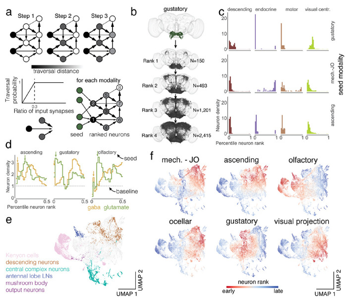
(a) We applied the information flow model for connectomes by Schlegel et al.20 to the connectome of the central brain neurons. Neurons are traversed probabilistically according to the ratio of incoming synapses from neurons that are in the traversed set. The information flow calculations were seeded with the afferent classes of neurons (including the sensory categories). (b) We rounded the traversal distances to assign neurons to layers. For gustatory neurons, we show a subset of the neurons (up to 1,000) that are reached in each layer. (c) For each sensory modality we used the traversal distances to establish a neuron ranking. Each panel shows the distributions of neurons of each super-class within the sensory modality specific rankings (see Ext. Data Fig. 6-1a for the complete set). (d) We assign neurons to neurotransmitter types and show their distribution within the traversal rankings similar to (c). The arrows highlight the sequence of GABA – glutamate peaks found for almost all sensory modalities (see Ext. Data Fig. 6-1b for the complete set). (e) We UMAP projected the matrix of traversal distances to obtain a 2d representation of each neuron in the central brain. Neurons from the same class co-locate (see also Ext. Data Fig. 6-2) (f) Neurons in the UMAP plot are colored by the rank order in which they are reached from a given seed neuron set. Red neurons are reached earlier than blue neurons (see Ext. Data Fig. 6-1c for the complete set).
U-map: https://codex.flywire.ai/app/rank_umap
Figure 7
Ocellar circuits and their integration with visual projection neurons. Link to figure 7
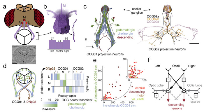
(a) Overview of the three ocelli (left, medial, right) which are positioned on the top of the head. Photoreceptors from each ocellus project to a specific subregion of the ocellar ganglion which are separated by glia (marked with black lines on the EM). (b) Renderings of the axons of the photoreceptors and their counts, and (c) OCG01, OCG02 and DNp28 neurons with arbors. “Information flow” from pre- and postsynapses is indicated by arrows along the arbors. (d) Connectivity matrix of connections between photoreceptors and ocellar projection neurons, including two descending neurons (DNp28). (e) Comparison of number of glutamatergic and cholinergic synapses from ocellar projection neurons onto downstream neurons colored by super-class (R=.65, p<1e-21). (f) Summary of the observed connectivity between ocellar projection neurons, visual projection neurons and descending neurons. Scale bar: 100 μm
Ocellar retinular cells:
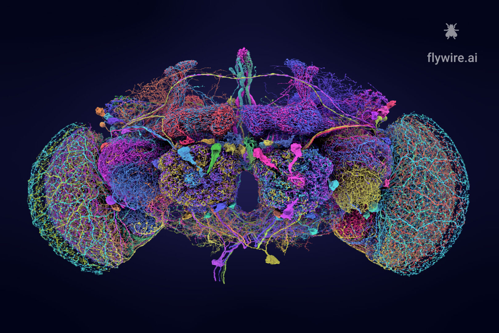
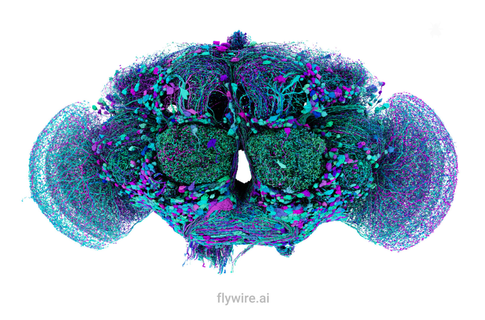
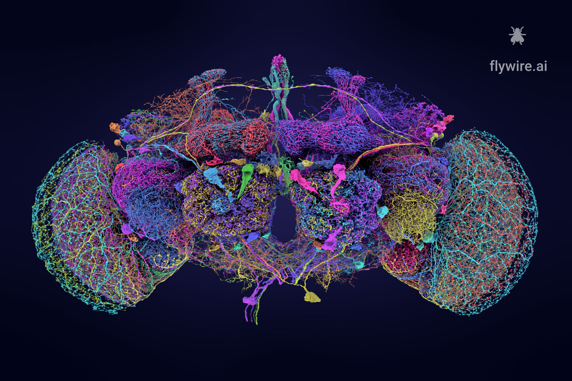
Thank you for reading Extended figures with Codex links and additional visualizations for the publication Neuronal wiring diagram of an adult brain. Now please enjoy some pretty pictures 🙂
Connectome Gallery
Who knew a fly could be beautiful?